A JOIN B == B JOIN A? (Just a Silly Question)

When Two SQL Queries Are the Same… But Not Really

The Question That Looked Silly

In 4th semester, DBMS was taught by Arpita ma'am. One day she was teaching joins, inner join, outer join, and conditions. Most people were copying notes. I was half listening.

And then I asked:

“Ma’am… if I change the order of joins, does the result change?”

She paused for a moment and smiled.

Then said:

“Read the Query Optimization and Relational Algebra chapter from Database System Concepts… and come tomorrow, we’ll discuss it.”

At that time, I thought it was just a textbook reference.

But I went back and opened the book, Database System Concepts by Abraham Silberschatz, Henry F. Korth, and S. Sudarshan, and read that chapter carefully.

The next day, when I came back, she didn’t just answer the question.

She walked me through:

how joins are commutative
how they are associative
how databases rewrite queries internally

And suddenly, the question didn’t feel simple anymore.

What I Found Instead

I realized something deeper:

Two SQL queries can look completely different and still be logically identical.

This is called Query Equivalence.

1️⃣ The Illusion of SQL

SELECT *
FROM A
JOIN B ON A.id = B.id
JOIN C ON B.id = C.id;

It looks sequential. But internally:

(A ⋈ B) ⋈ C  ≡  A ⋈ (B ⋈ C)
A ⋈ B ≡ B ⋈ A

2️⃣ The Real Problem

For n tables:

Possible join orders ≈ n!

For 10 tables → 3.6 million possibilities.

3️⃣ C++ Experiment (Step by Step Breakdown)

Instead of dropping one huge code block, I broke it into small steps.

Step 1: Headers

#include <bits/stdc++.h>
using namespace std;
using namespace std::chrono;

We use STL for data structures and chrono for nanosecond timing.

Step 2: Generate Data

vector<int> generateData(int size, int mod) {
    vector<int> v(size);

    for(int i = 0; i < size; i++) {
        v[i] = i % mod;
    }

    return v;
}

Step 3: Join A and B (Hash Join)

vector<int> joinAB(const vector<int>& A, const vector<int>& B) {

    unordered_set<int> setB(B.begin(), B.end());
    vector<int> result;

    for(int a : A) {
        if(setB.count(a)) {
            result.push_back(a);
        }
    }

    return result;
}

Step 4: Join Intermediate with C

vector<int> joinWithC(const vector<int>& AB, const vector<int>& C) {

    unordered_set<int> setC(C.begin(), C.end());
    vector<int> result;

    for(int x : AB) {
        if(setC.count(x)) {
            result.push_back(x);
        }
    }

    return result;
}

Step 5: Define Table Sizes

Imagine joining a small Users table (A), a medium Orders table (B), and a massive Logs table (C).

int sizeA = 1e4;   // small
int sizeB = 1e5;   // medium
int sizeC = 1e6;   // large

Step 6: Generate Tables

vector<int> A = generateData(sizeA, 5000);
vector<int> B = generateData(sizeB, 10000);
vector<int> C = generateData(sizeC, 20000);

Step 7: Case 1 → (A ⋈ B) ⋈ C

auto start1 = high_resolution_clock::now();

vector<int> AB = joinAB(A, B);
vector<int> result1 = joinWithC(AB, C);

auto end1 = high_resolution_clock::now();

Step 8: Case 2 → (C ⋈ B) ⋈ A

auto start2 = high_resolution_clock::now();

vector<int> CB = joinAB(C, B);
vector<int> result2 = joinWithC(CB, A);

auto end2 = high_resolution_clock::now();

Step 9: Measure Time

auto time1 = duration_cast<nanoseconds>(end1 - start1).count();
auto time2 = duration_cast<nanoseconds>(end2 - start2).count();

Step 10: Print Output

cout << "Case 1 Time: " << time1 << " ns\n";
cout << "Case 2 Time: " << time2 << " ns\n";
cout << "Slowdown: " << (double)time2 / time1 << "x\n";

📸 Output

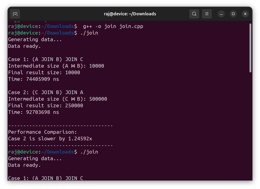
To verify the ground truth, I ran the program three times. The screenshots above are from those three runs.

4️⃣ Actual Results

Run 1:
Case 1: (A JOIN B) JOIN C
Intermediate size (A ⋈ B): 10000
Final result size: 10000
Time: 74405909 ns

Case 2: (C JOIN B) JOIN A
Intermediate size (C ⋈ B): 500000
Final result size: 250000
Time: 92703698 ns
Slowdown: 1.24592x

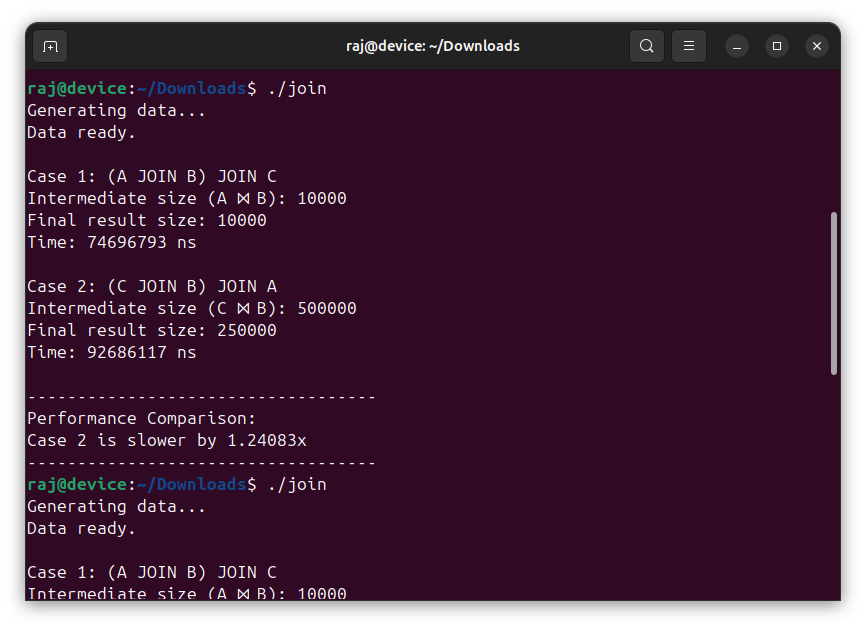
Run 2:
Case 1: (A JOIN B) JOIN C
Intermediate size (A ⋈ B): 10000
Final result size: 10000
Time: 74696793 ns

Case 2: (C JOIN B) JOIN A
Intermediate size (C ⋈ B): 500000
Final result size: 250000
Time: 92686117 ns
Slowdown: 1.24083x

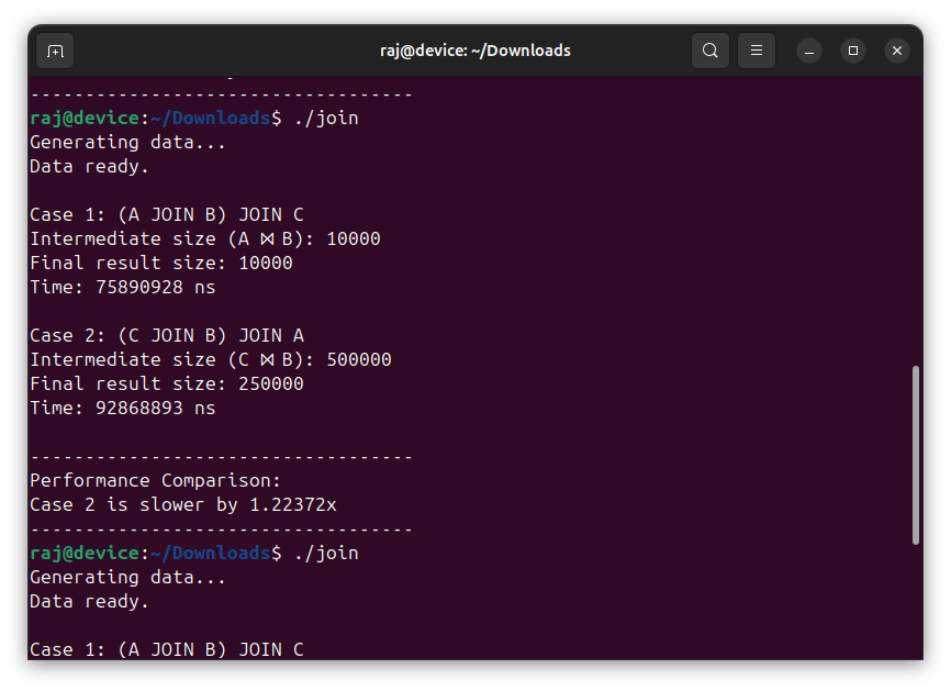
Run 3:
Case 1: (A JOIN B) JOIN C
Intermediate size (A ⋈ B): 10000
Final result size: 10000
Time: 75890928 ns

Case 2: (C JOIN B) JOIN A
Intermediate size (C ⋈ B): 500000
Final result size: 250000
Time: 92868893 ns
Slowdown: 1.22372x

5️⃣ What This Actually Means

At first glance:

“Only 1.22372x to 1.24592x difference... not huge?”

That first impression is misleading.

Intermediate (A ⋈ B): 10,000
Intermediate (C ⋈ B): 500,000   ← 50x bigger

6️⃣ Why Time Didn’t Explode

Because this experiment uses hash lookup:

unordered_set

So complexity behaves like:

O(n + m)

Not:

O(n × m)

7️⃣ The Hidden Truth

Join order affects intermediate size first and time second.

8️⃣ Real Databases Make This Worse

In real DBMS:

• Disk I/O
• Memory spilling
• Cache locality

That 1.24x can become:

10x → 100x → 1000x slowdown

9️⃣ Final Insight

🔟 Architect-Level Understanding

This is why every modern database uses a Cost-Based Optimizer (CBO). It relies on statistics to estimate these intermediate table sizes and picks the execution plan with the lowest computational "cost" before executing a single line of actual data.

Query equivalence → same result  
Join order → different intermediate sizes  
Intermediate size → performance impact  
CBO → chooses the lowest cost path

Closing Thought

The moment you realize SQL is not executed exactly as written, that is the moment you start thinking like a system architect.